Spline centrípeto de Catmull-Rom

En computación gráfica, el spline centrípeto de Catmull-Rom es una variante del interpolador cúbico de Hermite, formulada originalmente por Edwin Catmull y Raphael Rom,^[1]​ que puede calcularse utilizando un algoritmo recursivo propuesto por Barry y Goldman.^[2]​ Es un tipo de spline de interpolación definido por cuatro puntos de control ${\displaystyle \mathbf {P} _{0},\mathbf {P} _{1},\mathbf {P} _{2},\mathbf {P} _{3}}$ (por los que pasa), pero con la curva dibujada solo de ${\displaystyle \mathbf {P} _{1}}$ a ${\displaystyle \mathbf {P} _{2}}$.

Definición

Sea ${\displaystyle \mathbf {P} _{i}=[x_{i}\quad y_{i}]^{T}}$ un punto. Para un segmento de curva ${\displaystyle \mathbf {C} }$ definido por los puntos ${\displaystyle \mathbf {P} _{0},\mathbf {P} _{1},\mathbf {P} _{2},\mathbf {P} _{3}}$ y la secuencia de nodos ${\displaystyle t_{0},t_{1},t_{2},t_{3}}$, el spline centrípeto de Catmull-Rom se puede generar mediante:

${\displaystyle \mathbf {C} ={\frac {t_{2}-t}{t_{2}-t_{1}}}\mathbf {B} _{1}+{\frac {t-t_{1}}{t_{2}-t_{1}}}\mathbf {B} _{2}}$

donde

${\displaystyle \mathbf {B} _{1}={\frac {t_{2}-t}{t_{2}-t_{0}}}\mathbf {A} _{1}+{\frac {t-t_{0}}{t_{2}-t_{0}}}\mathbf {A} _{2}}$

${\displaystyle \mathbf {B} _{2}={\frac {t_{3}-t}{t_{3}-t_{1}}}\mathbf {A} _{2}+{\frac {t-t_{1}}{t_{3}-t_{1}}}\mathbf {A} _{3}}$

${\displaystyle \mathbf {A} _{1}={\frac {t_{1}-t}{t_{1}-t_{0}}}\mathbf {P} _{0}+{\frac {t-t_{0}}{t_{1}-t_{0}}}\mathbf {P} _{1}}$

${\displaystyle \mathbf {A} _{2}={\frac {t_{2}-t}{t_{2}-t_{1}}}\mathbf {P} _{1}+{\frac {t-t_{1}}{t_{2}-t_{1}}}\mathbf {P} _{2}}$

${\displaystyle \mathbf {A} _{3}={\frac {t_{3}-t}{t_{3}-t_{2}}}\mathbf {P} _{2}+{\frac {t-t_{2}}{t_{3}-t_{2}}}\mathbf {P} _{3}}$

y

${\displaystyle t_{i+1}=\left[{\sqrt {(x_{i+1}-x_{i})^{2}+(y_{i+1}-y_{i})^{2}}}\right]^{\alpha }+t_{i}}$

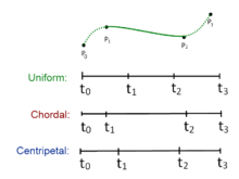
en el que ${\displaystyle \alpha }$ va de 0 a 1 para la parametrización de los nodos, y ${\displaystyle i=0,1,2,3}$ con ${\displaystyle t_{0}=0}$. Para el spline centrípeto de Catmull-Rom, el valor de ${\displaystyle \alpha }$ es ${\displaystyle 0.5}$. Cuando ${\displaystyle \alpha =0}$, la curva resultante es el spline uniforme de Catmull-Rom estándar; y cuando ${\displaystyle \alpha =1}$, el resultado es el spline cordal de Catmull-Rom.

Al conectar ${\displaystyle t=t_{1}}$ a las ecuaciones del spline ${\displaystyle \mathbf {A} _{1},\mathbf {A} _{2},\mathbf {A} _{3},\mathbf {B} _{1},\mathbf {B} _{2},}$ y ${\displaystyle \mathbf {C} }$ se muestra que el valor de la curva en ${\displaystyle t_{1}}$ es ${\displaystyle \mathbf {C} =\mathbf {P} _{1}}$. De manera similar, sustituir ${\displaystyle t=t_{2}}$ en las ecuaciones spline muestra que ${\displaystyle \mathbf {C} =\mathbf {P} _{2}}$ en ${\displaystyle t_{2}}$. Esto es cierto independientemente del valor de ${\displaystyle \alpha }$, ya que la ecuación de ${\displaystyle t_{i+1}}$ no es necesaria para calcular el valor de ${\displaystyle \mathbf {C} }$ en los puntos ${\displaystyle t_{1}}$ y ${\displaystyle t_{2}}$.

La extensión a puntos 3D se logra simplemente considerando ${\displaystyle \mathbf {P} _{i}=[x_{i}\quad y_{i}\quad z_{i}]^{T}}$ respecto a un punto 3D genérico ${\displaystyle \mathbf {P} _{i}}$ y

${\displaystyle t_{i+1}=\left[{\sqrt {(x_{i+1}-x_{i})^{2}+(y_{i+1}-y_{i})^{2}+(z_{i+1}-z_{i})^{2}}}\right]^{\alpha }+t_{i}}$

Ventajas

El spline centrípeto de Catmull-Rom tiene varias propiedades matemáticas deseables en comparación con la formulación original y otros tipos de splines de Catmull-Rom.^[3]​ En primer lugar, no formará un bucle ni una autointersección dentro de un segmento de curva. En segundo lugar, nunca genera cúspides dentro de un segmento de curva. En tercer lugar, sigue más estrictamente los puntos de control.^[4]​

Otros usos

En visión artificial, se ha utilizado el spline centrípeto de Catmull-Rom para formular un modelo activo para la segmentación. El método se denomina modelo de spline activo.^[5]​ El modelo está diseñado sobre la base del modelo de forma activo, pero utiliza un spline centrípeto de Catmull-Rom para unir dos puntos sucesivos (el modelo de forma activa utiliza una línea recta simple), de modo que el número total de puntos necesarios para representar una forma es menor. El uso del spline centrípeto de Catmull-Rom simplifica mucho el entrenamiento de un modelo de forma y permite una mejor manera de editar un contorno después de la segmentación.

Ejemplo de código en Python

La siguiente es una implementación del spline de Catmull-Rom en Python, que produce el gráfico que se muestra a continuación.

import numpy
import matplotlib.pyplot as plt


QUADRUPLE_SIZE: int= 4


def num_segments(point_chain: tuple) -> int:
    # Hay 1 segmento por cada 4 puntos, por lo que se debe restar 3 al número de puntos. 
    return len(point_chain) - (QUADRUPLE_SIZE - 1)


def flatten(list_of_lists) -> list:
    # P.ej. los puntos [[ 1, 2], [3], [4, 5]] to  [1, 2, 3, 4, 5] 
    return [elem for lst in list_of_lists for elem in lst]


def catmull_rom_spline(
    P0: tuple,
    P1: tuple,
    P2: tuple,
    P3: tuple,
    num_points: int,
    alpha: float= 0.5,
):
    """
    Compute the points in the spline segment
    :param P0, P1, P2, and P3: The (x,y) point pairs that define the Catmull-Rom spline
    :param num_points: The number of points to include in the resulting curve segment
    :param alpha: 0.5 for the centripetal spline, 0.0 for the uniform spline, 1.0 for the chordal spline.
    :return: The points
    """

     # Calcular t0 a t4. Luego, solo calcular los puntos entre P1 y P2.
     # Reformar linspace para que se pueda multiplicar por los puntos P0 a P3
     # y obtener un punto por cada valor de t.
    def tj(ti: float, pi: tuple, pj: tuple) -> float:
        xi, yi= pi
        xj, yj= pj
        dx, dy= xj - xi, yj - yi
        l= (dx ** 2 + dy ** 2) ** 0.5
        return ti + l ** alpha

    t0: float= 0.0
    t1: float= tj(t0, P0, P1)
    t2: float= tj(t1, P1, P2)
    t3: float= tj(t2, P2, P3)
    t= numpy.linspace(t1, t2, num_points).reshape(num_points, 1)

    A1= (t1 - t) / (t1 - t0) * P0 + (t - t0) / (t1 - t0) * P1
    A2= (t2 - t) / (t2 - t1) * P1 + (t - t1) / (t2 - t1) * P2
    A3= (t3 - t) / (t3 - t2) * P2 + (t - t2) / (t3 - t2) * P3
    B1= (t2 - t) / (t2 - t0) * A1 + (t - t0) / (t2 - t0) * A2
    B2= (t3 - t) / (t3 - t1) * A2 + (t - t1) / (t3 - t1) * A3
    points= (t2 - t) / (t2 - t1) * B1 + (t - t1) / (t2 - t1) * B2
    return points


def catmull_rom_chain(points: tuple, num_points: int) -> list:
    """
    Calculate Catmull-Rom for a sequence of initial points and return the combined curve.
    :param points: Base points from which the quadruples for the algorithm are taken
    :param num_points: The number of points to include in each curve segment
    :return: The chain of all points (points of all segments)
    """
    point_quadruples= (  # Prepare function inputs
        (points[idx_segment_start + d] for d in range(QUADRUPLE_SIZE))
        for idx_segment_start in range(num_segments(points))
    )
    all_splines= (catmull_rom_spline(*pq, num_points) for pq in point_quadruples)
    return flatten(all_splines)


if __name__== "__main__":
    POINTS: tuple= ((0, 1.5), (2, 2), (3, 1), (4, 0.5), (5, 1), (6, 2), (7, 3))  # Red points
    NUM_POINTS: int= 100  # Density of blue chain points between two red points

    chain_points: list= catmull_rom_chain(POINTS, NUM_POINTS)
    assert len(chain_points)== num_segments(POINTS) * NUM_POINTS  # 400 blue points for this example

    plt.plot(*zip(*chain_points), c="blue")
    plt.plot(*zip(*POINTS), c="red", linestyle="none", marker="o")
    plt.show()

Código ejemplo en Unity C#

using UnityEngine;

// a single catmull-rom curve
public struct CatmullRomCurve
{
	public Vector2 p0, p1, p2, p3;
	public float alpha;

	public CatmullRomCurve(Vector2 p0, Vector2 p1, Vector2 p2, Vector2 p3, float alpha)
   {
		(this.p0, this.p1, this.p2, this.p3)= (p0, p1, p2, p3);
		this.alpha= alpha;
	}

	// Evaluates a point at the given t-value from 0 to 1
	public Vector2 GetPoint(float t)
    {
		// calculate knots
		const float k0= 0;
		float k1= GetKnotInterval(p0, p1);
		float k2= GetKnotInterval(p1, p2) + k1;
		float k3= GetKnotInterval(p2, p3) + k2;

		// evaluate the point
		float u= Mathf.LerpUnclamped(k1, k2, t);
		Vector2 A1= Remap(k0, k1, p0, p1, u);
		Vector2 A2= Remap(k1, k2, p1, p2, u);
		Vector2 A3= Remap(k2, k3, p2, p3, u);
		Vector2 B1= Remap(k0, k2, A1, A2, u);
		Vector2 B2= Remap(k1, k3, A2, A3, u);
		return Remap(k1, k2, B1, B2, u);
	}

	static Vector2 Remap(float a, float b, Vector2 c, Vector2 d, float u)
    {
		return Vector2.LerpUnclamped(c, d, (u - a) / (b - a));
	}

	float GetKnotInterval(Vector2 a, Vector2 b)
    {
		return Mathf.Pow(Vector2.SqrMagnitude(a - b), 0.5f * alpha);
	}
}

using UnityEngine;

// Draws a catmull-rom spline in the scene view,
// along the child objects of the transform of this component
public class CatmullRomSpline : MonoBehaviour
{
	[Range(0, 1)]
    public float alpha= 0.5f;
	int PointCount=> transform.childCount;
	int SegmentCount=> PointCount - 3;
	Vector2 GetPoint(int i)=> transform.GetChild(i).position;

	CatmullRomCurve GetCurve(int i)
    {
		return new CatmullRomCurve(GetPoint(i), GetPoint(i+1), GetPoint(i+2), GetPoint(i+3), alpha);
	}

	void OnDrawGizmos()
    {
		for (int i= 0; i < SegmentCount; i++)
			DrawCurveSegment(GetCurve(i));
	}

	void DrawCurveSegment(CatmullRomCurve curve)
    {
		const int detail= 32;
		Vector2 prev= curve.p1;

		for (int i= 1; i < detail; i++)
        {
			float t= i / (detail - 1f);
			Vector2 pt= curve.GetPoint(t);
			Gizmos.DrawLine(prev, pt);
			prev= pt;
		}
	}
}

Código ejemplo en Unreal C++

float GetT( float t, float alpha, const FVector& p0, const FVector& p1 )
{
    auto d= p1 - p0;
    float a= d|d; // Dot product
    float b= FMath::Pow( a, alpha*.5f );
    return (b + t);
}

FVector CatmullRom( const FVector& p0, const FVector& p1, const FVector& p2, const FVector& p3, float t /* between 0 and 1 */, float alpha=.5f /* between 0 and 1 */ )
{
    float t0= 0.0f;
    float t1= GetT( t0, alpha, p0, p1 );
    float t2= GetT( t1, alpha, p1, p2 );
    float t3= GetT( t2, alpha, p2, p3 );
    t= FMath::Lerp( t1, t2, t );
    FVector A1= ( t1-t )/( t1-t0 )*p0 + ( t-t0 )/( t1-t0 )*p1;
    FVector A2= ( t2-t )/( t2-t1 )*p1 + ( t-t1 )/( t2-t1 )*p2;
    FVector A3= ( t3-t )/( t3-t2 )*p2 + ( t-t2 )/( t3-t2 )*p3;
    FVector B1= ( t2-t )/( t2-t0 )*A1 + ( t-t0 )/( t2-t0 )*A2;
    FVector B2= ( t3-t )/( t3-t1 )*A2 + ( t-t1 )/( t3-t1 )*A3;
    FVector C= ( t2-t )/( t2-t1 )*B1 + ( t-t1 )/( t2-t1 )*B2;
    return C;
}

Véase también

• Splines cúbicos de Hermite

Referencias

Enlaces externos

• Catmull-Rom curve with no cusps and no self-intersections – implementation in Java
• Catmull-Rom curve with no cusps and no self-intersections – simplified implementation in C++
• Catmull-Rom splines – interactive generation via Python, in a Jupyter notebook
• Smooth Paths Using Catmull-Rom Splines – another versatile implementation in C++ including centripetal CR splines

Esta página se editó por última vez el 13 mar 2024 a las 19:19.